


Control The Kinematic Chain, Control The Industrial Robot
If you want to make a modern robot move, you have to understand its kinematic chain. Understand how it is linked from its base frame to the TCP, and you'll know how it can function.

As a follow up to Kinematics Is At The Root Of Most Industrial Automation, this post will revisit the kinematic chain.
A couple key points:
All industrial machines have at their root, a “BASE” link, or “fixed” link.
The kinematic chain is a series of rigid bodies joined together by mechanisms, also known as joints.
Starting from the base link, each joint mechanism will equal 1 DOF Degree of Freedom. A modern 6 axis robot will have 6 DOF.
We are lucky to have the software we do today… A lot of the complex math behind this technology is calculated for us.

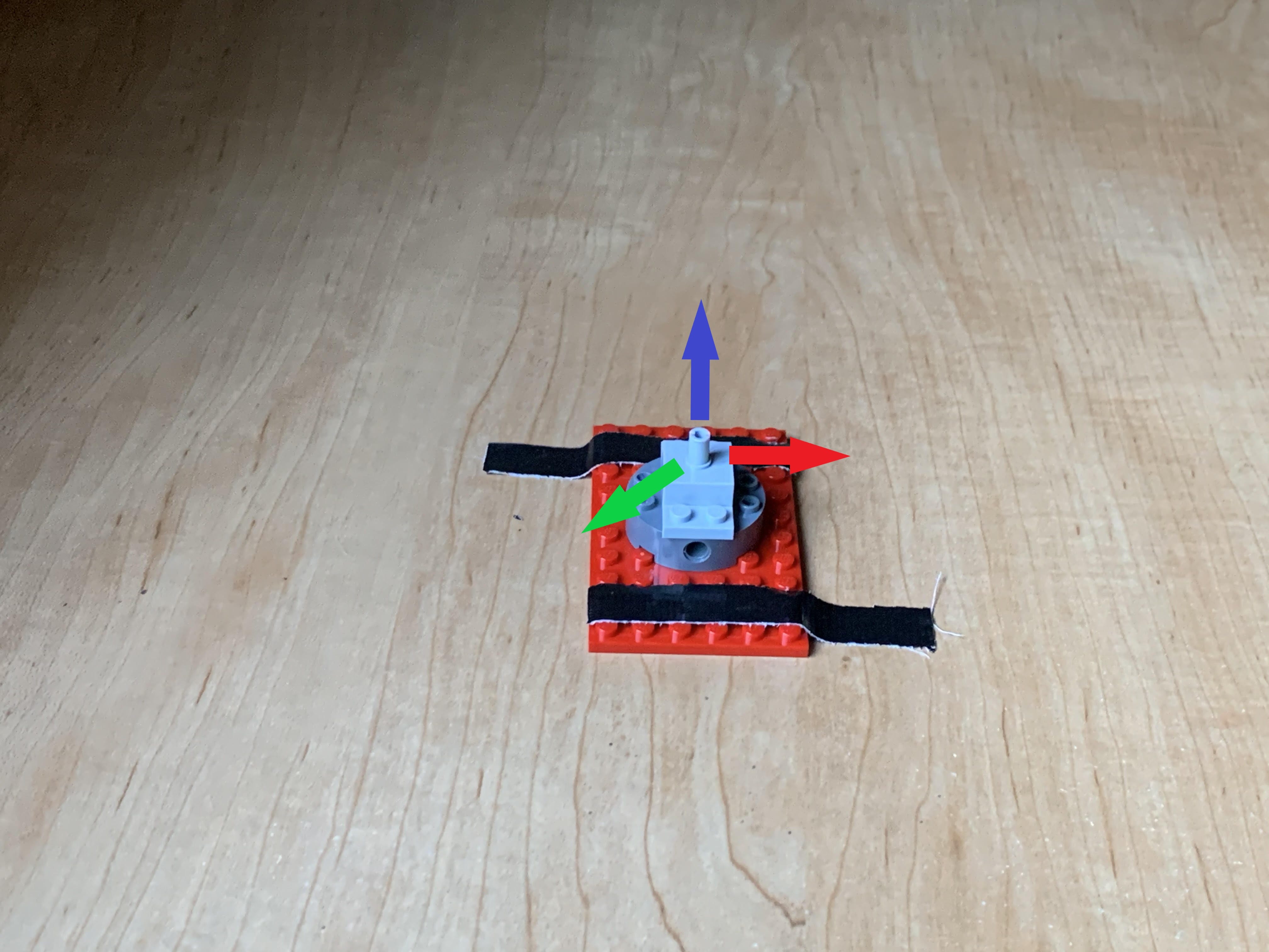
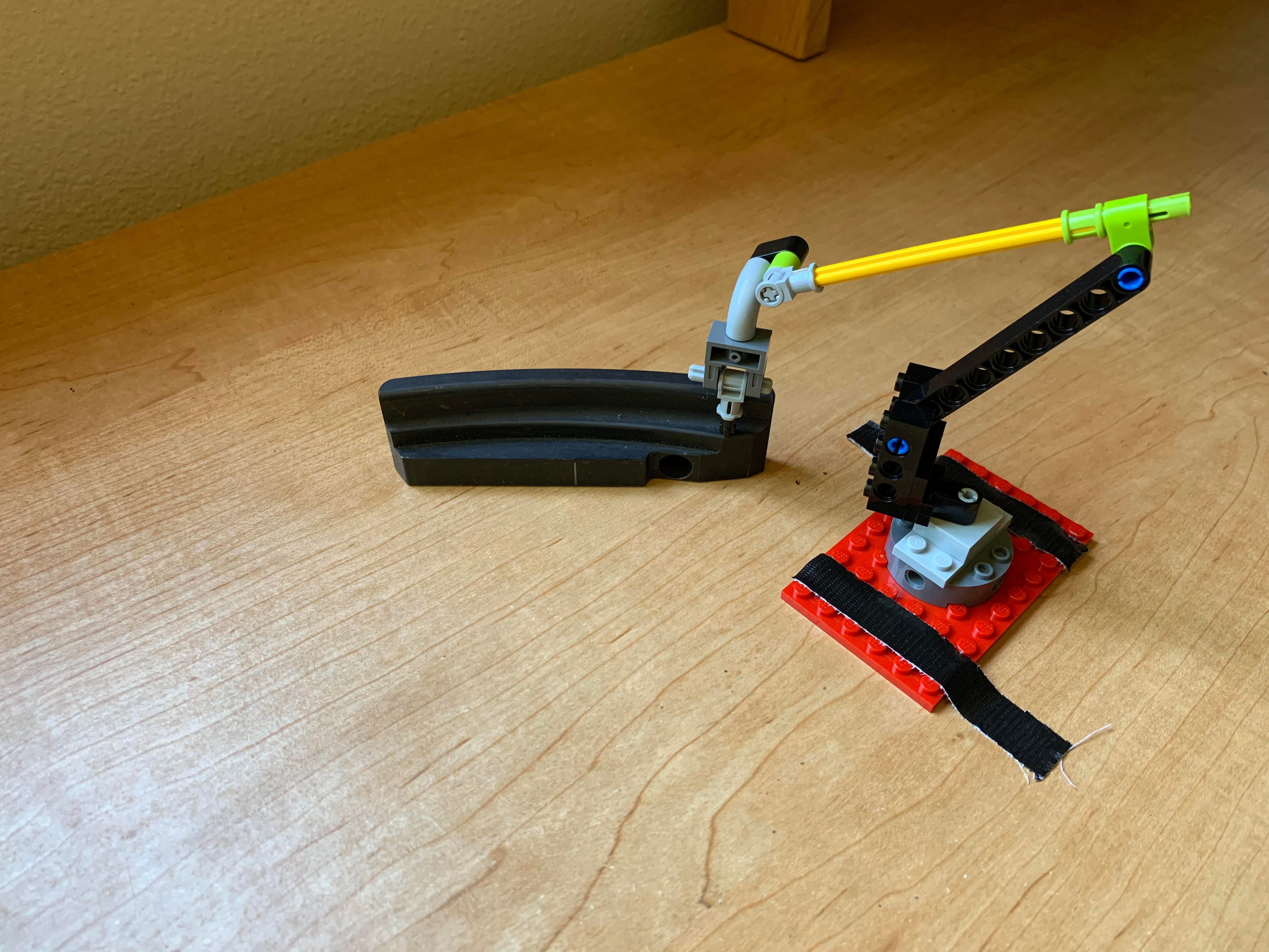
Building a Lego Kinematic Robot Chain
Base Joint / Fixed Joint / Base Frame
There will always be a fixed joint base frame. This is a specific location and orientation in space, and a key value to help us understand the kinematic chain.
It is fixed in relation to the larger world coordinates the robot exists within.
Joint 1 / DOF 1

Joint 2 / DOF 2

Joint 3 / DOF 3

Joint 4 / DOF

Joint 5 / DOF 5

Joint 6 / DOF 6
We will always build our chain such that the 6th axis rotates around Z, and the Z+ direction will face out from the robot joint.


Tool Mount Point
The tool mount point will be created at the end of the kinematic chain. It is represented by a XYZ location and orientation. Almost certainly the Tool Mount Point will be the exact same orientation as the Joint 6 DOF, maybe with an offset.

Tool Center Point
The Tool Center Point is essentially the tip of the tool we have attached to the end of the kinematic chain. In our scenario here, the Tool itself has no kinematics, it is simply an offset of the Joint 6 frame, along Z. It will share the same orientation as the tool mount point, but the length of the tool will create the offset about Z.
Note about TCP. It is the driver of linear targets. It is best to make a good connection with our real world tool, such that the TCP frame is related to a helpful place on the real world tool.
An example would be to understand where the exact tip of welding gun is located. This is in relation — via both location and orientation — to the tool mount point.

Two Ways to Control the Kinematic Chain
Note: A robot “task” is a programmed list of either joint targets or linear targets or combination.
Joint Programming
Joint programming is simply commanding the kinematic chain to drive each of its joints to a specific value within each of their ranges.
Typically a joint target is utilized at the beginning and/or end of a task. The power of a joint target is the ability to get the kinematic chain into a very specific configuration.
A good example would be at the end of a linear task, and we command a joint target to specifically unwind the 6th axis back to zero, which subsequently unwinds our attached paint gun and its paint lines.
Linear Programming
Linear programming is the method of setting the location and rotation of 1…n linear targets, which we then use to align the TCP of our robot. (See visual below for our planned robot targets)
The key difference between linear programming and joint programming, is the calculation of IK inverse kinematics.
Once we set our targets, we snap the TCP to the desired target location. The software calculates values for each joint from the TCP Inversely back down the kinematic chain to the base frame. There might be a couple configurations of the kinematic chain, which allow the robot to reach the target with its TCP.
This reduces our control of each of the joints, but allows us very specific command of the location we want to the TCP to try and reach. Imagine the TCP of a welding gun following a curve…
There are some inherent problems that can arise when linear programming.
Robot Singularities: During IK linear programming there will be times when the calculation of the kinematic chain, moving from one target to the next, reaches a point where there are infinite possibilities. This will result in an error and you must configure the targets and kinematic chain, such that it limits the possibilities.
Out of reach: All kinematic chains will have a limitation to what the can reach. We need to set linear targets in such a way that the kinematic chain we are working with can reach the target from its base frame to is TCP.
Milling A Golf Putter With A Lego Robot
Create Joint Position As Way Points
Joint Targets are great for home positions, entry/exit positions, and or start/end positions.
jHome

jStartEnd

Planned Robot Targets
These are the planned linear targets we would like our kinematic chain to follow. Our goal is to align the tool, via the TCP location, and drive it to these targets.
We plan the location and orientation of the targets in such a way that the TCP of the milling tool will cut the metal as we desire.

We Drive the TCP to Each target In Order to Check Kinematic Chain Reachability
Once We Confirm Reachability For Each Linear Target
We write a series of commands using each of the targets names. We start with the joint target waypoints, then with each of the linear targets, and back to the joint targets. They combine to create a cohesive robot task.
Main Program ()
MoveJoint jHome
MoveJoint jStartEnd
MoveLinear target1
MoveLinear target2
MoveLinear target3
MoveLinear target4
MoveLinear target5
MoveLinear target6
MoveLinear target7
MoveLinear target8
MoveLinear target9
MoveLinear target10
MoveLinear target11
MoveJoint jStartEnd
MoveJoint jHome
End
Final Program
